Injecting Structure into Diffusion Attention Through Its Prior
Every softmax row is an entropic transport plan with a cost and a reference measure. Conditioning writes to the cost. A vision-language model that writes to the measure gets an orthogonal, unbounded channel into a video diffusion model, and the gradient it receives is an exact advantage over chunks.
A softmax attention row is the exact solution of an entropic optimal transport problem, and that problem has two inputs: a cost, computed from the query and the keys, and a reference measure, the distribution the row is pulled toward before any cost is paid. Every standard way of conditioning a diffusion model writes to the cost. Masks, linear position biases and attention sinks write to the measure, and they are the only familiar mechanisms that do. We argue that the measure is the native channel for a vision-language model to inject structure into a video diffusion model: writing there is orthogonal to the computation inside each chunk, it is unbounded where the cost channel is capped by QK-normalization, and its gradient under the diffusion loss is an exact, sampling-free advantage over chunks. The coarse causal mask that a VLM chose in our experiments, and that improved chunked autoregressive generation, is the degenerate corner of this channel. The channel is needed because the diffusion model's own cost is dominated by position: its queries are noisy where their positions are exact, and once a row is peaked on nearby keys, the gradient that could teach it to look elsewhere is multiplied by an attention weight that is already zero.
The question we start from is a small engineering surprise. We generate video chunk by chunk with an autoregressive diffusion transformer; each new chunk attends, through a KV cache, to the chunks before it. When we let a vision-language model read the prompt and decide, per new chunk, which past chunks it may see, the generations get better. That should not happen to a model that already sees everything: an attention row can put as little weight on a chunk as it likes. So the mask is supplying something the model cannot produce for itself, and it is supplying it through the crudest possible interface, a binary pattern over chunks. We want to know what the non-crude version of that interface is, why the model needs it, and whether learning to use it is a reinforcement learning problem. A recent paper by Litman
- A softmax row minimizes expected cost plus $\tau$ times a KL divergence to a reference measure $\pi$. Conditioning changes the cost; a mask sets $\pi$ to zero on some keys. The soft version of a VLM mask is a per-chunk logit bias $\beta_b = \tau\log\pi_b$, and the row becomes a posterior: prior from the VLM, likelihood from the backbone. ()
- Attention over chunks factors into a gate over block potentials and a readout inside each block. A per-chunk bias moves only the gate, so the channel can be added to a frozen backbone, at no cost, in any block-sparse kernel. ()
- With QK-normalization the log-ratio of any two attention weights is bounded by $2G/\tau$. No signal entering through queries and keys can implement a mask or push a chunk below a fixed floor. The bias is a coordinate the backbone could not have learned to move. ()
- The gradient of the loss with respect to $\beta_b$ is $-(\sigma_b/\tau)A_b$, where $A_b$ is the advantage of chunk $b$. Every chunk's counterfactual readout is observed in one dense forward pass, so this is REINFORCE with an exact baseline and no sampling. Reinforcement learning proper is needed only across chunks, where the choice at chunk $n$ changes the state for chunk $n+1$. (, )
- The diffusion model needs the prior because its own attention is position-dominated for three reasons: the denoising target is local, a noisy query has an exact position but a corrupted content term, and the Fisher information of a peaked row, $(1-\|p\|^2)/\tau^2$, vanishes, so far keys stop receiving gradient however useful they are. Whether this is degeneracy depends on a measurement we have not made: whether any head retrieves an object across an occlusion. ()
- Attention sinks are the model's substitute for a null option that one-sided transport lacks. A hard mask must never remove the chunk that hosts the sink; the soft channel handles it automatically. ()
The Setting: A Mask That Should Not Help
Our model is a multimodal diffusion transformer
We found two things. First, when a vision-language model reads the prompt and emits, for each new chunk, a binary visibility pattern over past chunks, and we apply that pattern as a block-level causal mask, generations improve: objects that leave and re-enter the frame keep their identity more often, and long rollouts drift less.
The two observations are in tension. A model whose attention is diagonal is not using the distant chunks much, so masking them should change little. Yet masking helps. The resolution, which the rest of the article develops, is that the model cannot compute the thing the mask supplies: a content-based judgment about which past chunk matters now. The mask makes that judgment with a VLM that reads clean inputs, and injects the result at the only place where a judgment about keys can enter an attention row without going through the query.
A Softmax Row Has Two Inputs
Litman proves that the attention row $p$ for a query $q$ is the unique minimizer of
$$ J(p) = \sum_j p_j C_j - \tau H(p), \qquad C_j = -\langle q, k_j\rangle, $$over the probability simplex, where $H$ is Shannon entropy
The ALiBi case is the one to look at, because it exposes a second input hiding in the problem. The entropy term in $J$ is relative entropy to the uniform distribution. Nothing forces that choice. Replace it with relative entropy to an arbitrary reference measure $\pi$ on the keys:
$$ p^\star = \arg\min_{p \in \Delta}\ \sum_j p_j C_j + \tau\, \mathrm{KL}(p \,\|\, \pi). $$The stationarity condition is $C_j + \tau(\log p_j - \log \pi_j + 1) = \lambda$, so
$$ p^\star_j \;\propto\; \pi_j\, e^{s_j/\tau} \;=\; \exp\!\big((s_j + \tau \log \pi_j)/\tau\big). $$The reference measure enters as an additive logit bias $\tau \log \pi_j$, and every additive logit bias is a reference measure. ALiBi is the measure $\pi_j \propto e^{-\gamma|i-j|/\tau}$. A causal mask is the measure that is zero on the future. The VLM's chunk mask is the measure that is zero on the chunks it rejected. This is the content of : an attention row has a cost input and a measure input, and the two are written to by disjoint sets of mechanisms.
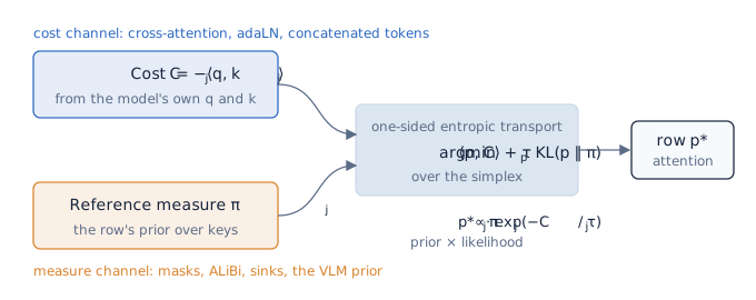
Conditioning, in all its forms, is on the cost side. Cross-attention to a text encoder, adaptive layer norm driven by a timestep or a caption embedding, and VLM features concatenated as extra tokens all change $q$ and $k$, and therefore $C$. The backbone must learn to translate the signal into scores. The measure side is different in kind: it is a prior over keys that the row multiplies in before the backbone's own evidence is weighed. In Bayesian terms, $p^\star_j \propto \pi_j\, e^{s_j/\tau}$ is a posterior with prior $\pi$ and likelihood $e^{s/\tau}$. Conditioning changes the likelihood. A mask changes the prior.
Seen this way, the VLM's binary mask is a dogmatic prior: it puts zero mass on some chunks, and no evidence from the backbone can restore them. The soft version, a per-chunk bias $\beta_b = \tau \log \pi_b$ with $\pi_b$ positive, is a prior that a strong enough score can overrule. lets you move between the two. We call $\beta_b$ the measure channel, and the rest of the article is about why it is the right place for a VLM to write.
The Measure Channel Leaves the Chunk Alone
The reason a chunk-level prior is cheap, and safe to add to a frozen model, is an identity that every online-softmax kernel already uses. Partition the keys into blocks $B_1, \dots, B_n$ and define for each block a potential and a readout:
$$ \phi_b(q) = \tau \log \sum_{j \in B_b} e^{s_j/\tau}, \qquad o_b(q) = \sum_{j \in B_b} \frac{e^{s_j/\tau}}{\sum_{l \in B_b} e^{s_l/\tau}}\, v_j . $$Then the full attention output is a gate over blocks applied to the block readouts:
$$ \mathrm{Attn}(q) = \sum_b \sigma_b(q)\, o_b(q), \qquad \sigma(q) = \mathrm{softmax}\big(\phi(q)/\tau\big). $$This is associativity of the exponential sum. Now add a bias $\beta_b$ to every score in block $b$. Inside the block the softmax is invariant to a constant shift, so $o_b$ does not move. The potential shifts by exactly $\beta_b$, so the gate becomes $\sigma_b \propto \exp((\phi_b + \beta_b)/\tau)$. A per-chunk prior is a modification of the gate and nothing else ().
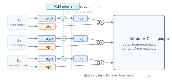
Three consequences follow. The channel composes with a frozen backbone: within each chunk the model computes exactly what it computed before, so nothing it learned about local structure is disturbed. The channel is free: a per-block additive bias is what a block-sparse attention kernel already supports, and it costs nothing beyond the addition. And the channel is the same object as the hard mask: set $\beta_b = -\infty$ on the rejected chunks and you recover the pattern the VLM chose in our experiments, so whatever the mask was doing, the bias can do with a continuous dial.
Under QK-Norm the Cost Channel Is Bounded
One might ask why the backbone could not learn to do this itself through conditioning. Give it the VLM's features as extra tokens; let the queries and keys adjust. The answer is that the cost channel has a ceiling that the measure channel does not. Modern diffusion transformers normalize queries and keys before the dot product
and a chunk of $|B_b|$ keys out of $N$ keeps a share of at least $(|B_b|/N)\, e^{-2G/\tau}$ no matter what the queries and keys contain. The cost channel can attenuate a chunk by a bounded factor and can never exclude it (). The measure channel has no such floor: $\beta_b$ is added after normalization, outside the bound.
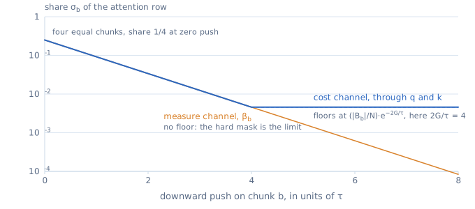
The bound matters less for its numerical value than for what it says about the mechanism. To suppress a chunk through the cost, the backbone must rotate the content of queries and keys, which are also carrying every other function those vectors serve. The bias is a coordinate independent of all of them. It is not a knob the backbone could have learned to turn through its inputs; it is a knob that did not exist in its parameterization. This is the precise sense in which the measure channel is native: it is one of the two inputs the row has, and the model's training has only ever written to the other one.
The Prior's Gradient Is a Chunk Advantage
The second half of Litman's paper concerns the backward pass. Let $c = \sum_j p_j v_j$ be the context vector, $L$ a downstream loss, $g = \nabla_c L$, and define the marginal utility of key $j$ as $u_j = -\langle g, v_j\rangle$: the reward for putting more weight on it. Then the gradient of the loss with respect to a score is
$$ \frac{\partial L}{\partial s_j} = -\frac{p_j}{\tau}\,\big(u_j - \mathbb{E}_p[u]\big), $$which is REINFORCE with the expected utility as baseline
Sum this over a chunk. Since $\beta_b$ shifts every score in $B_b$ by the same amount, $\partial L/\partial \beta_b = \sum_{j \in B_b} \partial L/\partial s_j$, and a short calculation () gives
$$ \frac{\partial L}{\partial \beta_b} = -\frac{\sigma_b}{\tau}\, A_b, \qquad A_b = -\langle g,\; o_b - c\rangle . $$$A_b$ is the advantage of chunk $b$: positive when the chunk's readout $o_b$ lies downhill of the current output $c$ along the loss gradient, in which case the prior on the chunk should rise, and negative when it lies uphill (). The advantages are mean-zero under the gate, $\sum_b \sigma_b A_b = 0$, so shifting every chunk's prior together is a null direction, as it should be.
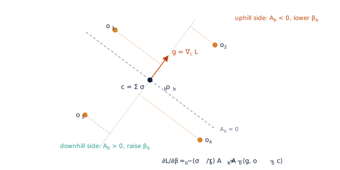
Two things about this gradient are unusual for a reinforcement learning signal. It is exact: a single dense forward pass through the diffusion model evaluates every chunk's readout, including the ones the prior is currently suppressing, so there is no Monte Carlo variance and no need to roll out alternatives. And it is cheap: $o_b$ and $c$ are already materialized by any attention kernel that processes keys in blocks. A VLM head that outputs $\beta$ can be trained by ordinary backpropagation through a frozen backbone, and the signal it receives is the advantage of each chunk under the current policy.
What the Diffusion Model Cannot Compute
We now return to the puzzle. A model that can put arbitrarily little weight on a chunk should not benefit from having the chunk removed. It benefits because the weight it puts on chunks is not a judgment about content; it is, to a first approximation, a function of position. We see three reasons, of increasing depth, and the third is where Litman's geometry does real work.
Locality Is Learned ALiBi
Video latents are strongly correlated across nearby positions in space and time, and the denoising target at most noise levels is well predicted by a local neighborhood. The minimum-mean-square denoiser of a locally correlated field is a local filter, and a transformer trained to be one learns a cost that increases with distance. In the variational framework this is a learned ALiBi: a linear-in-distance penalty on the regularizer, induced through rotary position encoding rather than written in by hand. Analyses of video diffusion transformers report exactly this: heads sort into spatially local and temporally local types
Noisy Queries, Exact Positions
The second reason is specific to diffusion and, we think, underappreciated. The query is computed from a noisy latent, $x_t = \alpha_t x_0 + \sigma_t \epsilon$. Its content term is a mixture of signal and noise, $\alpha_t\langle q_0, k\rangle + \sigma_t\langle \epsilon, k\rangle$, and the second part carries no information about which key is relevant. Its position term, carried by the rotary phase, is exact at every noise level. So at high noise the cost is position-dominated by construction, before any learning has happened (). The model is not failing to compute a content-based judgment at the early steps; it has nothing to compute it from.
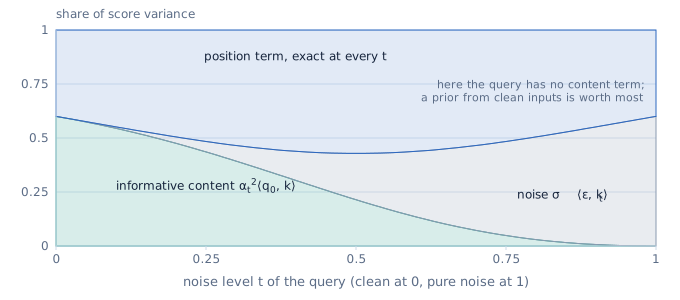
This also says where the prior is worth most. A VLM reads the prompt and the clean past chunks; it can judge which chunk holds the object that is about to re-enter the frame, at every noise level. The measure channel carries that judgment into the rows whose own content term is noise. The prior should therefore be strongest at high noise and fade as the query becomes informative, which suggests making the VLM head a function of the noise level or scheduling $\beta$ against it.
A Peaked Row Stops Learning
The third reason is dynamical. Litman shows that the standard gradient with respect to the scores is the natural-gradient direction $u$ pushed through the Fisher information matrix of the row
The trace of $F$ is $(1 - \|p\|^2)/\tau^2$, a function of the Rényi-2 entropy of the row, and it goes to zero as the row becomes peaked. Since $F$ is positive semidefinite, $\|\nabla_s L\| \le (1 - \|p\|^2)\,\|u\|/\tau$, and per key, $|\partial L/\partial s_j| = (p_j/\tau)\,|A_j|$. A key with small attention receives small gradient however large its advantage. shows the consequence: once the position term has made the row local, the one distant key that would help cannot be learned, because its learning signal is multiplied by an attention weight that is already near zero.
The process is self-reinforcing. The position term is the easiest gain, so it is learned first. Once it dominates, the Fisher metric has collapsed along every non-local direction, and the content subspace of the query-key map stops receiving signal from distant keys. This is attention entropy collapse
Is This Degeneracy?
Whether the diagonal pattern means the attention has degenerated depends on two measurements we have not yet made, and we want to be precise about what they are. The first is the difference between attention weight and attention effect. The weight on a distant key may be small while its contribution to the output is large, if its value vector is large and aligned with what the layer needs
The second is the existence of retrieval heads. In language models most heads are local and a small minority carry long-range retrieval; removing that minority destroys long-context ability while leaving everything else intact
Sinks Are the Missing Null Option
One more feature of the transport problem explains a pattern that appears alongside the diagonal. The source marginal in one-sided transport is fixed at one: every row must place a full unit of mass on the keys. There is no option to decline. The unbalanced version of the problem
a softmax that can sum to less than one over the real keys. The proposal to add such a logit has been made for language models
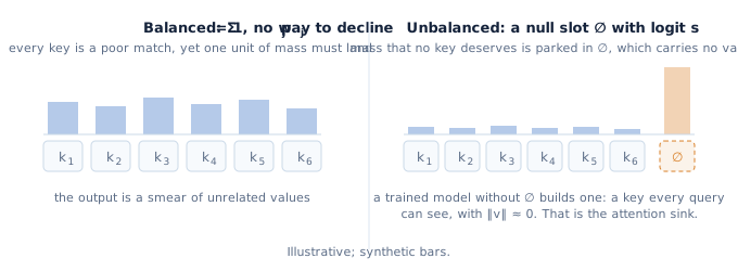
This has three consequences for the channel. A hard mask must not remove the chunk or tokens that host the sink; if it does, the surplus mass is forced onto unrelated keys and the output degrades, which is the failure that streaming language models hit when the first token leaves the window
Where Reinforcement Learning Enters
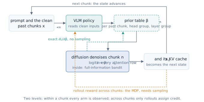
Is learning to use the channel a reinforcement learning problem? Litman's result is easily summarized as attention doing reinforcement learning, and it is worth being exact about what that means. Within one row, the softmax is a policy over keys, the utility is a reward, and backpropagation is the policy gradient. But the reward of every arm is observed, so this is a full-information bandit: no exploration, no variance, no bootstrapping. The same is true one level up. The VLM's $\beta_b$ parameterizes a prior over chunks, and showed that its gradient is an exact advantage computed from readouts that a single dense pass produces. If the VLM's output is continuous, learning it is supervised learning in disguise.
Reinforcement learning proper enters across chunks (). The prior chosen for chunk $n$ changes the chunk that is generated, which changes the cache, which is the state for chunk $n+1$. That is a Markov decision process whose state is the prompt, the chunks so far and their cache, whose action is the prior table for the next chunk, and whose reward is the quality of the rollout. Credit for a visibility decision at chunk $n$ that pays off at chunk $n+4$ cannot come from the one-step gradient; it needs rollouts. The action is low-dimensional, a few scalars per past chunk per head group, and the backbone is frozen, so group-sampled policy optimization
This suggests a two-stage recipe. First, train the VLM's prior head by the exact gradient, against a loss that requires long-range information: distillation toward a teacher that sees every past chunk in clean form, rather than the teacher-forced denoising loss, which the local solution already satisfies. Second, fine-tune by rollouts with a reward that sees drift, for instance a judge of object identity across the generated video, using the stage-one advantage as the baseline. If the VLM must emit a discrete mask, for instance as text, the dense pass still gives every chunk's readout, so its advantage can serve as the reward for the discrete choice instead of a noisy rollout score.
The gain we observed from the VLM's mask has two possible sources, and they point at different dials. It could come from semantic selection, or merely from showing the model less of a drifted past. Masks of equal sparsity chosen at random, by recency alone, and by the VLM separate the two: if the VLM's mask does not beat recency, the information being injected is trust rather than content, and the right dial is the null logit, a decaying trust in the past, rather than a prior over chunks.
The Full Set of Dials
Everything above concerned one dial, the per-chunk bias. The transport problem has three ingredients, cost, regularizer and marginal constraints, and each admits a modification that an external model could write. We list them so the choice is explicit.
| Dial | Ingredient | Form | Meaning | Cost to implement |
|---|---|---|---|---|
| $\beta_b$ | reference measure | logit $+\,\beta_b$ on block $b$ | how much chunk $b$ matters now | a block bias in the kernel; nothing |
| $\kappa_b$ | cost, rank one | logit $+\,\langle q, \kappa_b\rangle$ on block $b$ | when chunk $b$ matters, as a function of what is asked | one scalar per query and block, precomputed |
| $\tau_b$ | regularizer strength | temperature inside block $b$ | how broadly to read within the chunk | a scale inside the block |
| $s_0$ | marginal, unbalanced | an extra null logit | how much to distrust every past chunk | one extra column |
| $b_b$ | target marginal | column constraint, Sinkhorn | how much total mass chunk $b$ receives across queries | iterations inside attention |
We would start with $\beta_b$, add $\kappa_b$ if the prior needs to depend on the query, and add $s_0$ if the equal-sparsity comparison points at trust rather than content. We would not pursue the target marginal; it is the one dial that cannot be added to a fused attention kernel. A zero-training variant of $\beta_b$ is also available: the VLM's own attention from the prompt onto frames of the past chunks is itself a transport plan, and its mass on chunk $b$ can be used as $\pi_b$ directly.
Limitations
Our experimental claim is qualitative and comes from one internal model; the retrieval-head probe and the equal-sparsity mask comparison have not been run, and we say so where they appear. The bound in is loose in practice: trained gains can make $2G/\tau$ large, so the floor may be low; its force is in the mechanism it describes rather than its value. The three explanations of diagonal attention are not exclusive and we have not measured their relative weights. The exactness of the one-step gradient depends on evaluating every chunk's readout in a dense pass, which is affordable at training time but is not what a sparse inference kernel does. And the claim that a VLM supplies a content term the model lacks assumes the VLM's judgment is good; a wrong prior is overruled by a strong score, which is the argument for the soft channel, but it still costs something.
Related Work
The variational view of softmax goes back to maximum-entropy inference and was made exact for attention by Litman
Appendix: Derivations
Reference measure. Minimize $\sum_j p_j C_j + \tau\sum_j p_j(\log p_j - \log \pi_j)$ subject to $\sum_j p_j = 1$. The Lagrangian condition is $C_j + \tau(\log p_j - \log\pi_j + 1) - \lambda = 0$, so $\log p_j = \log \pi_j - C_j/\tau + \mathrm{const}$ and $p_j \propto \pi_j e^{s_j/\tau}$. The objective is strictly convex on the simplex, so this is the unique minimizer. A global rescaling of $\pi$ cancels; a zero in $\pi$ makes the KL term infinite off its support, which is the hard mask.
Block decomposition. $\sum_{j} e^{s_j/\tau} = \sum_b e^{\phi_b/\tau}$ by definition of $\phi_b$, and $\sum_j e^{s_j/\tau} v_j = \sum_b e^{\phi_b/\tau} o_b$ by definition of $o_b$; divide. Adding $\beta_b$ to all $s_j$ with $j \in B_b$ multiplies $e^{\phi_b/\tau}$ by $e^{\beta_b/\tau}$ and leaves the within-block normalized weights unchanged.
Bounded log-ratio. $|s_j - s_l| \le |\langle q, k_j\rangle| + |\langle q, k_l\rangle| \le 2 G_q G_k$ by Cauchy-Schwarz, and $\log p_j - \log p_l = (s_j - s_l)/\tau$. Summing $p_j \ge p_{\max} e^{-2G/\tau}$ over a block and using $p_{\max} \ge 1/N$ gives the floor.
Chunk advantage. With $\partial L/\partial s_j = -(p_j/\tau)(u_j - \mathbb{E}_p[u])$ and $\partial s_j/\partial \beta_b = \mathbf{1}[j \in B_b]$,
$$ \frac{\partial L}{\partial \beta_b} = -\frac{1}{\tau}\sum_{j\in B_b} p_j\big(u_j - \mathbb{E}_p[u]\big) = -\frac{\sigma_b}{\tau}\Big(\bar u_b - \mathbb{E}_p[u]\Big), \qquad \bar u_b = \sum_{j \in B_b}\frac{p_j}{\sigma_b}\, u_j . $$Since $\sum_{j\in B_b}(p_j/\sigma_b)\, v_j = o_b$ and $u_j = -\langle g, v_j\rangle$, we have $\bar u_b = -\langle g, o_b\rangle$ and $\mathbb{E}_p[u] = -\langle g, c\rangle$, so $A_b = \bar u_b - \mathbb{E}_p[u] = -\langle g, o_b - c\rangle$. Mean-zero: $\sum_b \sigma_b \bar u_b = \sum_j p_j u_j = \mathbb{E}_p[u]$.
Fisher trace and gradient bound. $\mathrm{tr}(\mathrm{diag}(p) - pp^\top) = \sum_j p_j - \sum_j p_j^2 = 1 - \|p\|^2$, and $1 - \|p\|^2 = 1 - e^{-H_2(p)}$ with $H_2$ the Rényi-2 entropy. $F \succeq 0$ because it is a covariance, that of the one-hot indicator under $p$, so its operator norm is at most its trace, and $\|\nabla_s L\| = \tau\|F u\| \le \tau\,\mathrm{tr}(F)\,\|u\| = (1 - \|p\|^2)\|u\|/\tau$.
Null option. Append a key with score $s_0$ and value $0$ to the transport problem; the minimizer over the enlarged simplex is the softmax over $(s_0, s_1, \dots, s_m)$, and the output $\sum_{j\ge 1} p_j v_j$ carries less than one unit of value mass. A real key with $v \approx 0$ that every query can see implements the same thing with $s_0 = \langle q, k_{\mathrm{sink}}\rangle$.
Footnotes
References
Citation
Xiao, “Injecting Structure into Diffusion Attention Through Its Prior”, Han Xiao’s Blog, 2026.
@article{xiao2026injecting,
  author  = {Han Xiao},
  title   = {Injecting Structure into Diffusion Attention Through Its Prior},
  journal = {Han Xiao’s Blog},
  year    = {2026},
  note    = {https://blog.hanxiao.run/attention-prior-channel/}
}